Monte Carlo Analysis
This is an experimental feature. That means we're still working on finishing it. There may be bugs, missing functionality or incomplete documentation, and we may decide to remove the feature in a future release. If you have any feedback, please comment on the dedicated feedback issue.
What Does This Report Do?
The Monte Carlo Analysis report helps you answer one of the biggest money questions there is: "If I stop working and start living off my savings, will the money last?"
Nobody knows what the stock market will do next year, let alone over the next 30 years. So instead of guessing once, this report guesses thousands of times. It replays your retirement over and over - 5,000 times by default - and in each replay the market has different luck: some replays hit a crash early on, some enjoy a long boom, most land somewhere in between.
At the end it tells you a simple, powerful number: in what percentage of those replays did your money last as long as you needed it to? If your plan survives in 85% of the replays, that's a much more honest answer than any single prediction could give you.
This report is a planning aid, not financial advice, and not a prediction. It can't know the future - it can only show you how your plan holds up across many possible futures.
Turning the Report On
Monte Carlo Analysis is an experimental feature, so it's switched off until you enable it:
- Open Settings from the sidebar.
- Click Show advanced settings.
- Open Experimental features and acknowledge the warning.
- Tick Monte Carlo Analysis Report.
Adding the Report to Your Dashboard
- Go to Reports in the sidebar.
- Click Add new widget and choose Monte Carlo analysis.
- A card appears on your dashboard showing your success rate and a small chart. Click the card to open the full report.
- After changing any settings in the full report, click Save widget so your setup is remembered next time.
The report works immediately with sensible example numbers filled in, so you can explore how it behaves before entering your own figures.
Setting Up Your Plan
The configuration area at the top of the report is organized into six tabs.
Plan Details
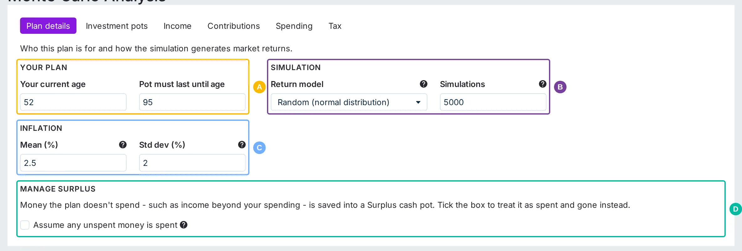
The tab is organized into four small groups - A. Your plan, B. Simulation, C. Inflation and D. Manage surplus:
-
Your current age and Pot must last until age - these two numbers define the period being tested. If you're 40 and want the money to last until you're 95, the report simulates 55 years.
-
Return model - how the simulation invents each year's investment returns:
- Random (normal distribution): each year's return is drawn randomly around the expected return and volatility you set on each pot. Think of it as a weighted coin flip, year after year. Every pot lives through the same simulated market year - a good year is good for all your pots, scaled by each pot's volatility - so two pots holding the same investments earn the same return.
- Historical returns, shuffled: instead of invented numbers, each simulated year is a real year from US market history (1928 onwards), picked in random order. Real crashes like 1931 and 2008 are in the deck, and each sampled year brings its own actual US inflation with it, so high-inflation years keep their high-inflation markets.
- Historical returns, in blocks: each replay is stitched together from runs of consecutive real years. A replay starts at a random year of US market history and usually carries on to the next real year, so a crash is followed by the years that actually followed it; every so often it jumps to a different point in history and carries on from there. Each year brings its own actual US inflation with it. This keeps the multi-year patterns that shuffling throws away, while still giving you thousands of different replays instead of one per starting year. A run that reaches the end of the data carries on from 1928.
- Historical sequences (replay): each replay is actual history, played in order from a different starting year - "what if you retired in 1929?", "what if you retired in 1972?", and so on. Each replayed year brings its own actual US inflation with it. This is the strictest test of bad timing, because real crashes and recoveries happen in their true order.
All three historical models only take real returns for pots with an asset mix - an allocation preset, or a complete custom mix. A Custom pot always draws random returns around its own expected return and volatility, which is useful for assets history can't stand in for, such as an annuity or property. If every pot is Custom, a historical model's returns behave just like the random model's - though spending still follows each historical year's real inflation.
-
Simulations - how many replays to run (1,000 to 10,000). More replays give steadier numbers but take slightly longer. When using historical sequences, this field is disabled because there is exactly one replay per historical starting year.
-
Block length (years) - only shown for Historical returns, in blocks. How many consecutive real years are replayed, on average, before a replay jumps to a different point in history (1 to 30). Longer blocks keep more of history's multi-year patterns, such as a crash and its slow recovery; shorter blocks mix history up more, and a length of 1 behaves like the shuffled model. The default of 10 years is a common choice.
-
Inflation - Mean (%) - the average yearly rise in prices. When set, your planned spending grows with it so your spending power keeps up. Leave it blank to take exactly the same amount every year. With a historical return model, the two inflation inputs are replaced by an Adjust spending with inflation checkbox: each simulated year then uses that year's actual US inflation, keeping inflation and market returns paired the way they really were.
-
Inflation - Std dev (%) - real-world inflation bounces around from year to year rather than staying fixed. When set, each simulated year draws its own inflation rate around the mean, separately in every replay. The default of 2% is roughly how much US inflation has varied in recent decades; set it to 0 to use the fixed mean rate every year. Only used by the random return model.
-
Manage surplus - Assume any unspent money is spent - what happens to money the plan doesn't spend in a year, such as income beyond your spending. Unticked (the default), a Surplus cash pot holds everything the plan doesn't spend and is drawn on first when spending needs funding; tick it and unspent money simply leaves the plan. See Income for the details.
Investment Pots
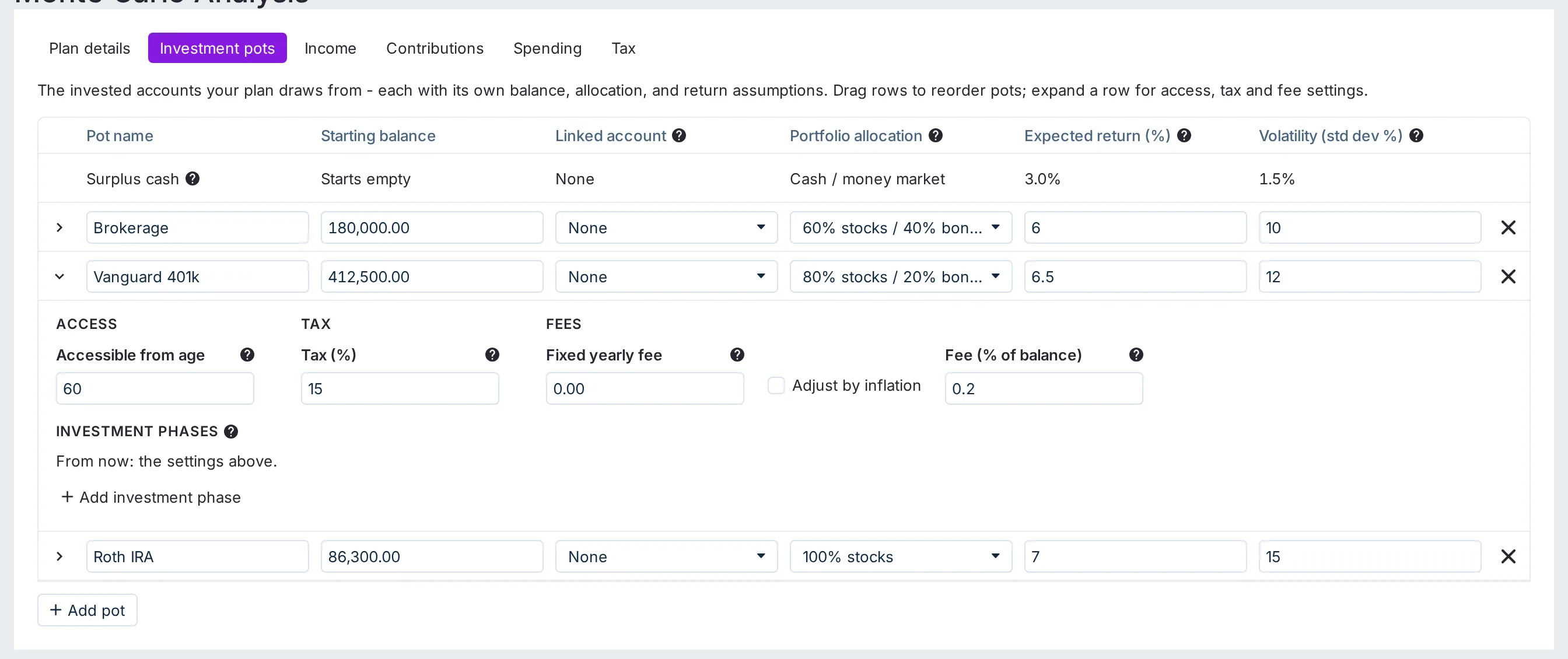
A pot is a chunk of invested money - a pension or retirement account, an investment account, a savings account. You can model one pot or several, each with its own settings:
-
Pot name - anything you like, such as "Pension".
-
Starting balance - how much is in the pot today. Enter it by hand, or use Linked account below to keep it up to date automatically.
-
Linked account - link the pot to one of your accounts and its starting balance becomes that account's live balance, so the plan tracks reality without re-typing numbers. Typing a starting balance manually unlinks the pot and keeps your typed value - useful for what-if questions like "how big would this pot need to be?" - and you can re-link it any time with the picker.
-
Portfolio allocation - a one-click preset that fills in a typical expected return and volatility for a given mix of stocks and bonds. A pot that's 100% stocks tends to grow faster but swings harder; a cash pot barely moves in either direction. You can always override the numbers, which switches the pot to Custom. If none of the presets match your portfolio, pick Custom mix and enter your own stock, bond and cash percentages in the pot's expanded settings - the allocation must total 100%, and until it does the pot falls back to the expected return and volatility you enter. With a historical return model, the mix (a preset's or a custom one) is also the pot's real asset mix - its stock, bond and cash shares take each sampled year's actual S&P 500, 10-year Treasury and T-bill returns, and the return and volatility cells show the mix's measured history instead of editable assumptions (only Custom pots, and a custom mix under the random model, keep using their typed values, via random draws).
-
Expected return (%) - the average yearly growth you expect from this pot, before inflation.
-
Volatility (std dev %) - how much the returns swing from year to year. Two pots can have the same average return, but the one with higher volatility is riskier: bad early years can do damage that a smooth ride would avoid. Click the arrow at the start of a pot's row to expand its additional settings, organized into groups:
-
Allocation - Stocks / Bonds / Cash (%) - only shown for Custom mix pots: the pot's own asset shares, as described under Portfolio allocation above. Picking Custom mix in the allocation dropdown expands the row automatically, seeded with the shares of the preset you were on. The allocation must total 100% - a warning appears until it does, and in the meantime the pot uses its typed return and volatility.
-
Access - Accessible from age - some pots can't be touched until a certain age; retirement accounts in many countries work this way. Leave this blank if the pot is available now. A locked pot stays invested and keeps growing - it just can't pay your bills until you reach the access age.
-
Tax - Tax (%) (or Taxable portion (%) with the bands model) - how withdrawals from this pot are taxed; see Tax below. Leave at 0 for tax-free pots.
-
Fees - what this pot costs you each year, charged at the end of every simulated year:
- Fixed yearly fee - the sum of fixed costs like adviser or platform fees, as an amount. Tick Adjust by inflation if the fee will rise with prices over time (untick it for a contractually flat fee, which shrinks in real terms).
- Fee (% of balance) - percentage charges like fund management fees, taken from the pot's end-of-year balance - e.g. 0.22 for a typical index fund platform.
-
Investment phases - change what the pot is invested in, and what it costs, from a given age. The pot's own allocation, return, volatility and fees apply until the first phase begins; each phase sets a From age and its own allocation (a preset, a custom mix, or hand-typed return and volatility) and fees. Transition decides how the pot gets there: At once switches on that birthday, while Gradually from the previous phase moves in a straight line from the previous phase's start age and arrives at the age you set. That makes a glide path one row: a pot that is 100% stocks today with a phase of "60% stocks / 40% bonds, from age 65, gradually" shifts a little more into bonds every year and is at 60/40 on your 65th birthday. A later "Cash, at once, from 80" would then move the whole pot to cash at 80. Phases work with every return model - the historical models blend each year's real returns by that year's mix - and the run drill-in shows each pot's allocation year by year once a pot has phases. Switching investments is free in the simulation; any dealing costs or tax on the switch are not modelled.
Drag a pot's row to reorder the list - the order matters if you choose to drain pots one at a time (see Spending below).
The access age setting is what lets the report model the classic "bridge gap": retiring at 48 with a big pension you can't open until 57, and a smaller pot that has to carry you across those nine years. If the bridge pot runs dry too soon, the plan fails - even though the pension money exists.
Income
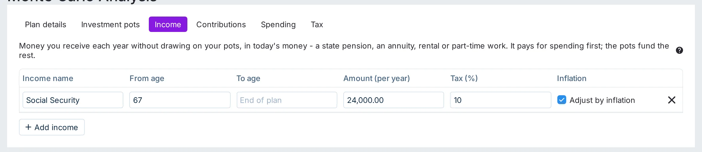
Income streams are money you receive each year without drawing on your pots - a state pension, a defined-benefit pension, an annuity, rental income, or part-time work in early retirement. They matter because they pay for your spending first: with £40,000 of yearly spending and a £12,000 state pension, the pots only need to fund £28,000, and the withdrawal rules and the failure test both work on that smaller amount. Each stream has:
- Income name - anything you like, such as "State pension".
- From age and To age - the years the income arrives, inclusive at both ends. Leave From age blank to start now, and To age blank to keep receiving it until the end of the plan.
- Amount (per year) - the gross yearly amount, in today's money, before any tax.
- Tax (%) (or Taxable portion (%) with the bands model) - how the income is taxed, exactly as for pot withdrawals: an effective rate under the flat model, or the share that counts as taxable income under the bands model. Under the bands model, income fills your lower tax bands first, so any pot withdrawal in the same year is taxed at the correct, higher marginal rate.
- Adjust by inflation - tick this for income that rises with prices (most state pensions do); untick it for a fixed amount, such as a level annuity, which buys a little less each year as prices rise.
Income you don't need is unspent: once the year's contributions paid from it and its spending are covered, anything left is dealt with according to the Manage surplus setting on the Plan Details tab:
- Assume any unspent money is spent unticked (the default for new plans): a Surplus cash pot sits at the top of your pots. Income beyond your spending is saved into it at the start of the year (so it earns that year's return), and it is always the first pot drawn on when spending needs funding. It starts empty and holds cash - no access age, no tax, no fees - and its settings can't be changed in the pots list. Tick the setting to remove it, along with any contributions paid into it.
- Ticked: unspent money leaves the plan - it isn't invested and doesn't help later years. The run drill-in and the cashflow chart both point out unspent income so it doesn't go unnoticed, and you can route specific amounts into a pot with a contribution whose Paid from is that income stream. Plans saved before this setting existed keep this behaviour; untick the box to add the Surplus cash pot.
A plan whose income covers its spending doesn't need the pots at all, and empty pots are not a failure on their own - the plan only fails in a year whose spending can't be paid for from income and pots together.
Contributions

If you're still earning, you can model the money you add to your pots each year - pension deposits or brokerage savings, anything that tops up a pot on a regular basis. Each contribution has:
- Contribution name - anything you like, such as "Pension contributions".
- Into pot - the pot the money is paid into. A pot can receive any number of contributions, and contributions can go into a pot that is still locked for withdrawals - the access age only controls when money can come out.
- Paid from - where the money comes from. Outside the plan (the default) means money the simulation doesn't otherwise know about. Choosing one of your income streams instead pays the contribution out of that income: it is capped at what the stream brings in that year, and it is zero in years the stream pays nothing. Tick Before tax for a workplace pension or salary sacrifice - the contribution is deducted before the income's tax is worked out, so it lowers that year's tax bill.
- From age and To age - the years the contribution runs, inclusive at both ends. Leave From age blank to start now, and To age blank to keep contributing until the end of the plan.
- Amount (per year) - how much is added each year, in today's money. The money is paid in at the start of each year, so it earns that year's investment return.
- Adjust by inflation - tick this if the contribution will grow with prices over time (for example, a percentage of a salary that keeps pace with inflation). Untick it for a fixed amount, which buys a little less each year as prices rise.
Contributions pair naturally with a spending phase set to 0: while you're working, salary covers your costs and the plan only accumulates; from your retirement age, contributions stop and spending begins.
Spending
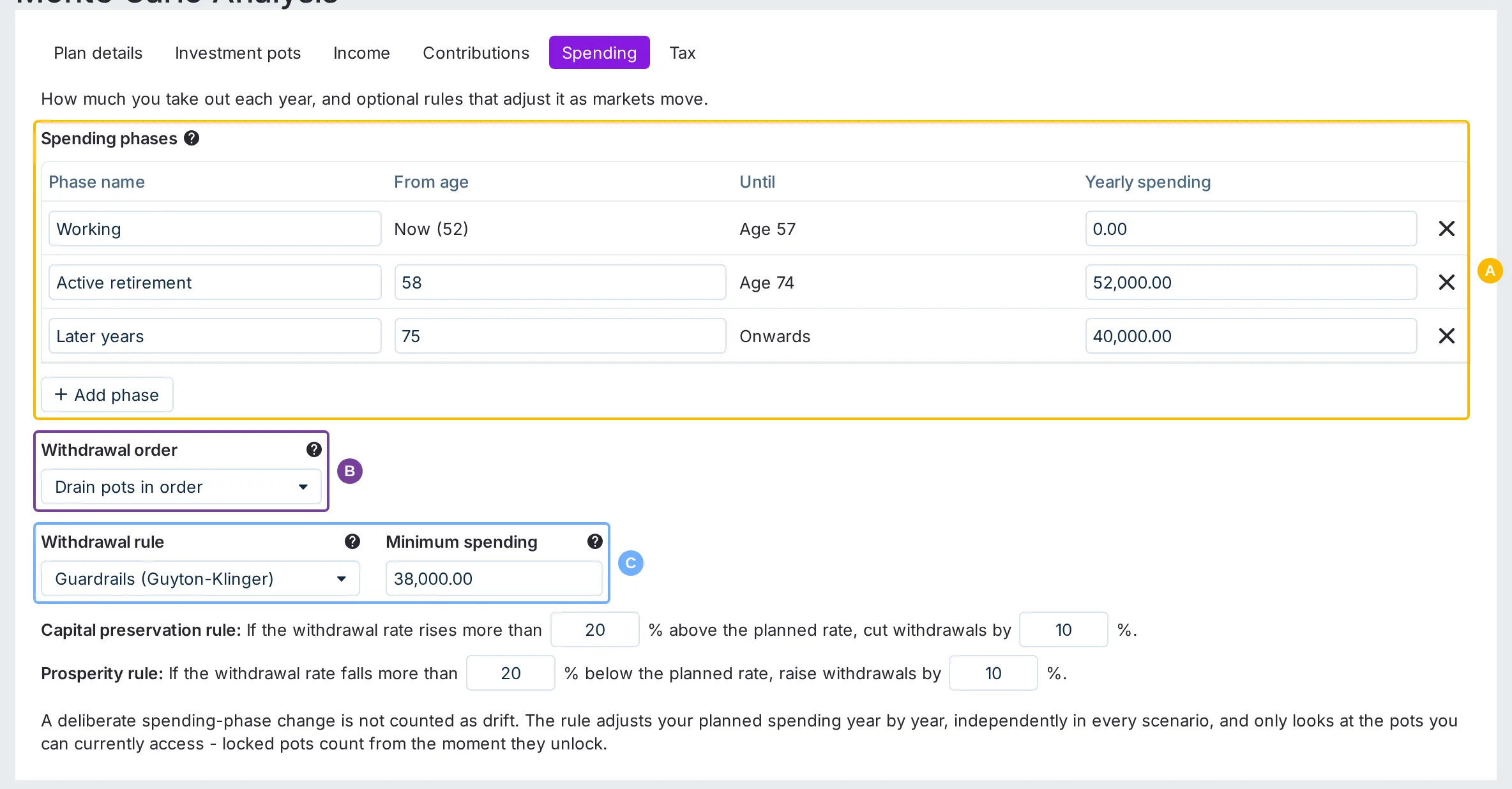
- A. Spending phases - how much you take out each year to live on. You can keep it simple with a single phase, or split your plan into phases with different amounts - for example, $30,000 a year for your first 10 years of retirement while you're travelling, then $20,000 a year onwards. Each phase sets a yearly amount from a chosen age until the next phase begins; the first phase always starts now. Amounts are in today's money - the inflation settings on the Plan Details tab are applied on top, so "$20,000 from age 65" always means $20,000 of today's spending power.
- B. Withdrawal order - only matters if you have more than one pot:
- Split proportionally across pots: each year's withdrawal is taken from all pots in proportion to their size, so they shrink together.
- Drain pots in order: empty the first pot in your list before touching the next - for example, spend your taxable account first and let the pension keep compounding. Pots that haven't reached their access age are skipped until they unlock.
- Spend from the best performer first: each year, the withdrawal comes from the pot that earned the highest return last year. This is the classic "bucket strategy" instinct: after a stock crash, live off your cash and give the crashed pot time to recover; in a boom year, spend from stocks and leave the cash reserve alone. The first year (when there's no track record yet) uses your listed order, and locked pots are skipped here too.
- Keep pots at their target mix: each pot's share of your starting balances becomes its target weight, and withdrawals come from whichever pots have grown above their target - most overweight first - pulling the portfolio back toward the mix you chose. This behaves like the best-performer option in booms and crashes (trim stocks after a good run, spend cash and bonds after a crash) but without slowly drifting your money into low-growth pots, because it always steers back to your chosen mix. If you want a permanent cash buffer, give the cash pot the share you want to maintain and this order will keep it topped up in spirit - by spending it only when it's above its target share.
- C. Withdrawal rule and Minimum spending - see the next section.
The inflation settings that grow your spending over time live on the Plan Details tab.
Tax

Withdrawing money from a pension or a taxable account usually costs more than the amount you get to spend. The Tax tab lets the simulation account for that: your yearly spending is always what you keep after tax, and the simulation withdraws extra to cover the tax bill. Two models are available:
- Flat rate per pot (the default) - each pot gets one effective tax rate on its withdrawals, set in the pots table. A tax-free account is 0%. For a pension with a tax-free portion, blend it with your expected income tax rate - for example, 25% tax-free plus 20% tax on the rest works out around 15%. For a taxable investment account, estimate the effective rate on your typical withdrawal. This is deliberately simple and works for any country - you own the number.
- Tax bands (progressive) - enter your own tax brackets: yearly income thresholds and the rate above each one (your tax-free allowance is simply the first band at 0%). Each pot then declares its Taxable portion (%) - how much of a withdrawal counts as taxable income: a pension with a 25% tax-free lump portion is 75, a tax-free account is 0, and a taxable account is roughly the share of each withdrawal that is gains. The bands apply to each year's combined taxable withdrawals across all pots, and the thresholds are in today's money - they rise with inflation in the simulation.
With either model, the run drill-in shows each year's gross withdrawal with the tax paid underneath, so you can see exactly what your spending actually costs.
Income streams are taxed the same way, using their own rate or taxable portion. Under the bands model the year's income is banded first and the pot withdrawals are taxed as the slice above it - so a taxable pension that uses up your tax-free allowance makes every withdrawal that year cost more, just as it does in real life.
This is a deliberate approximation, not a tax calculator. It doesn't track capital-gains cost basis, model frozen thresholds, or know any country's actual rules - and tax law changes every year. Treat the rates and bands as your own honest estimates.
Withdrawal Rules Explained
By default, the simulation withdraws the same (inflation-adjusted) amount every year, no matter what the market does. Real retirees usually don't behave that way - in a bad stretch they tighten their belts, and in a good stretch they allow themselves a bit more. Withdrawal rules teach the simulation to do the same.
All the rules share a few ideas:
- Your spending phases set the planned amounts. The rules wake up in your first year of planned spending: that year takes the planned amount (only a Minimum spending set higher than it can override that), and from the next year onward the rule adjusts what's actually taken - independently in every replay, reacting to how that replay is going. Zero-spend years (for example, working years before retirement) neither trigger nor move the rules. A cut or raise carries across phase boundaries: if the rule cut your spending by 10% during a rough patch, the next phase's amount starts 10% lower too.
- Rules usually improve your success rate by cutting spending in bad times, but that safety isn't free - you get it by living on less. Keep an eye on the Median total withdrawn stat to see what a rule costs you in income.
- Rules only see the wealth you can actually spend. If a pension is locked until its access age, it doesn't earn you spending raises while a bridge pot pays the bills - the rules watch the accessible pots, and the pension starts counting the moment it unlocks.
If you set a Minimum spending, your yearly spending never drops below that amount, no matter what the rule says - it is the lowest amount you need to live on, so when the rule cuts below it the plan is lifted back up to it and that is what gets spent. Income streams count towards it, so the pots only withdraw enough to top your spending up to the floor - a 12,000 floor with a 10,000 state pension means the pots never pay less than 2,000. It only applies in years you actually plan to spend - a spending phase set to 0 (for example, years before retirement while your salary covers your costs) takes nothing. Like your spending phases, it's an amount in today's money - it rises with inflation so its spending power holds steady.
Guardrails (Guyton-Klinger)
Think of this as pay cuts and pay rises. The rule watches what percentage of your remaining money you're withdrawing each year. If your pots shrink so much that the percentage drifts well above where your plan says it should be, you take a pay cut (for example, 10% less). If your pots race ahead and the percentage falls well below it, you get a pay rise. You set how far the percentage must drift before the rule reacts, and how big the adjustment is. The drift is measured against your planned spending path, so moving into a deliberately higher or lower spending phase doesn't count as drift by itself - only market-driven changes do.
Ratcheting (Kitces)
The optimist's rule: withdrawals only ever go up, never down. If your balance stays above a threshold (for example, 1.5 times what you started with) for several years in a row, you give yourself a raise. If markets fall, your spending simply stays where it is - the rule never cuts.
Floor & Ceiling (Bengen)
Instead of a fixed amount, each year you withdraw a fixed percentage of whatever the pots are currently worth - so spending naturally falls in bad years and rises in good ones. The percentage is set in your first year of planned spending (your planned amount divided by your accessible wealth at that point), and the withdrawal is then kept within a floor and a ceiling around your planned (inflation-adjusted) amount so it can't swing too wildly.
Boundaries
A simpler version of Guardrails: you set an upper and lower limit on the withdrawal percentage directly. Above the upper limit, spending is cut; below the lower limit, it's increased.
Reading the Results
By default, every money figure in the results is shown in today's money - what the amounts would actually be worth in terms of today's prices, discounted by each replay's own inflation path. Untick Show values in today's money to see the raw future amounts instead; they'll look much bigger over long horizons, but most of that is inflation rather than real growth. The success rate and failure ages are the same either way.
The Headline Numbers

- Success rate - the big number: the percentage of replays in which every year's spending was paid for, from income and pots together. There's no single "right" target, but many planners aim for 80–90%. (Running the pots down to nothing isn't a failure by itself - only a year whose spending goes unfunded is.)
- Median ending balance - in the middle-of-the-road replay, how much was left at the end.
- Median total withdrawn - how much income the middle replay actually paid you over the whole period. Especially useful when comparing withdrawal rules.
- Chance of running out of money - the flip side of the success rate.
- Typical failure runs out at - among the replays that failed, the typical age the money ran out.
The Portfolio Performance Chart
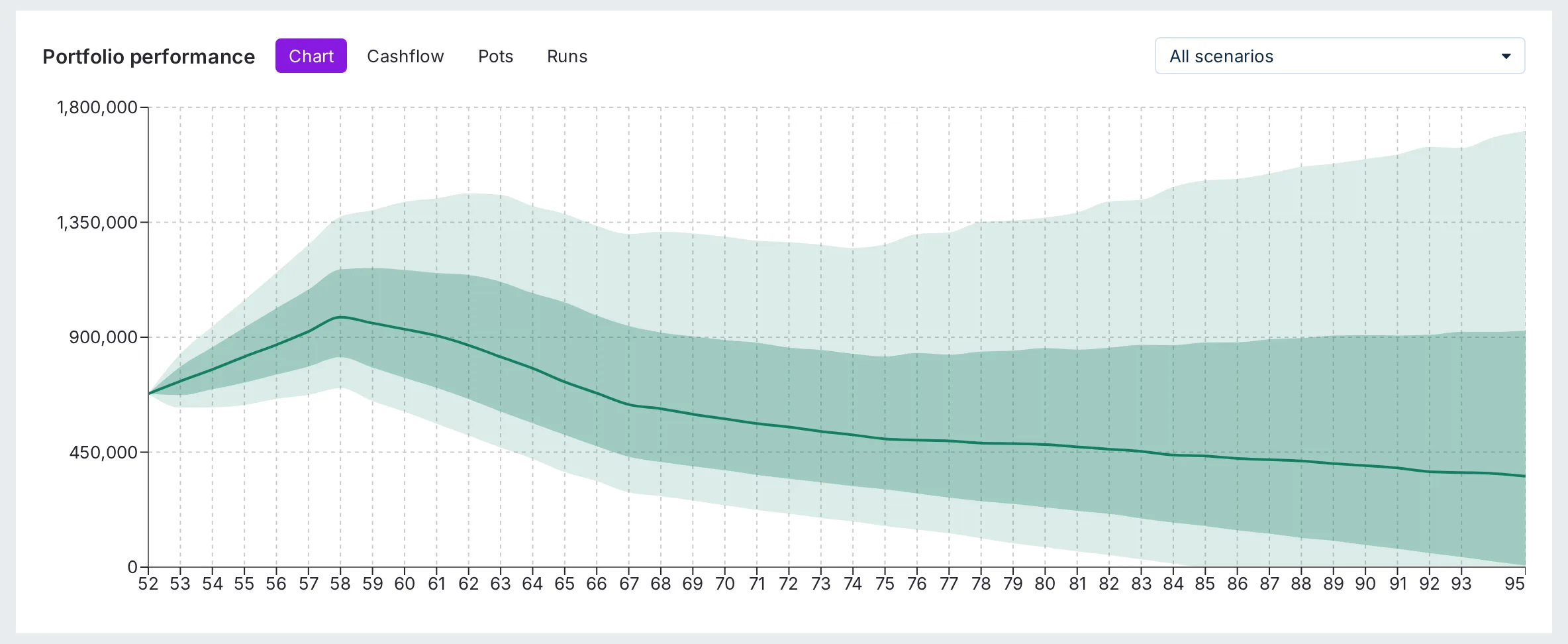
The chart shows your total balance from your current age to your target age - but instead of one line, it shows the whole range of futures at once:
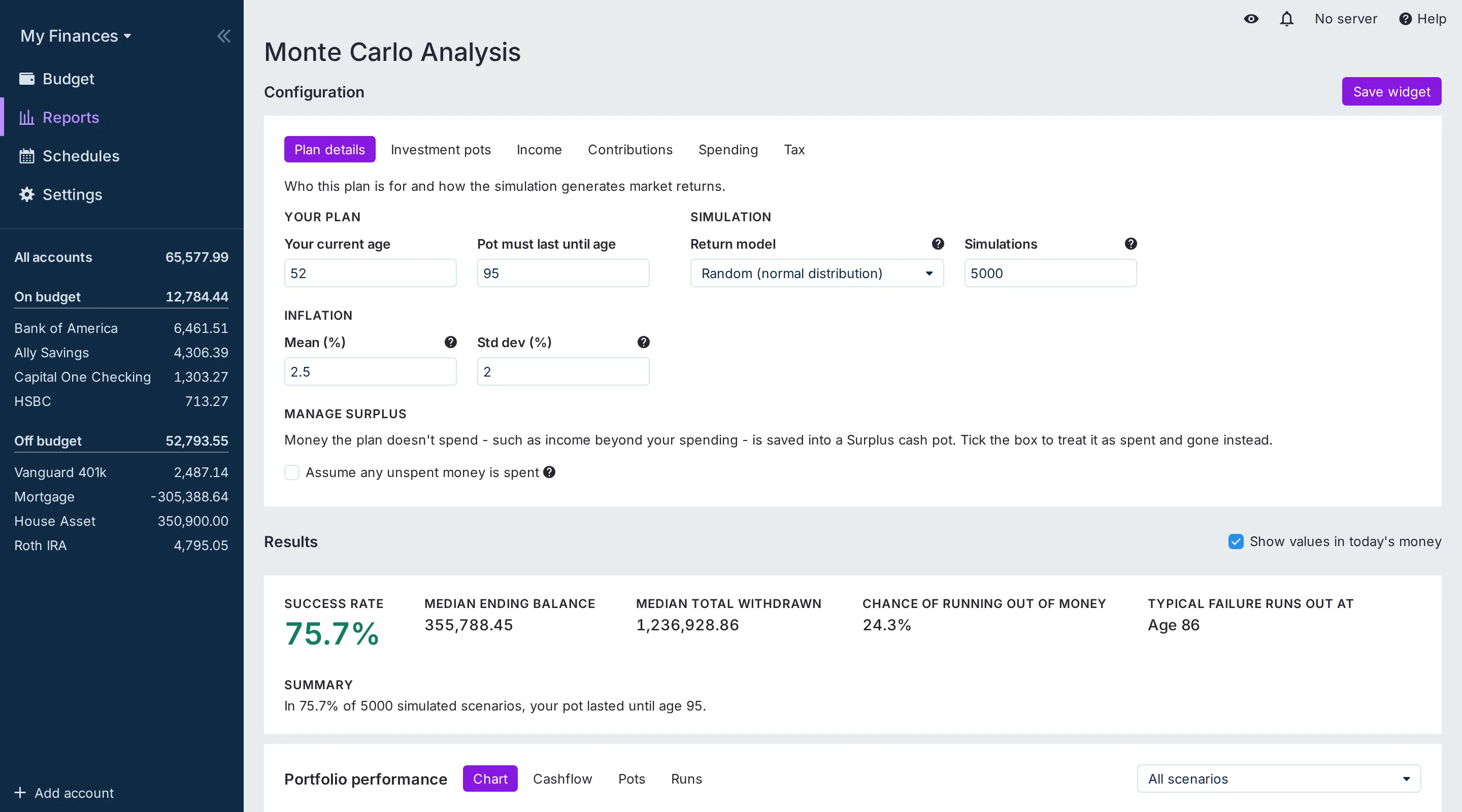
- The lighter band covers 80% of all replays - at any age, 8 out of 10 replays landed inside it.
- The darker band covers the middle half of replays.
- The line is the median: half the replays did better, half did worse.
The dropdown above the chart switches views. Single worst run shows the one unluckiest replay in full. The Worst-case, Pessimistic, Median and Optimistic views each trace a single percentile - for example, the pessimistic line is the level that 70% of replays stayed above.
The Cashflow Chart
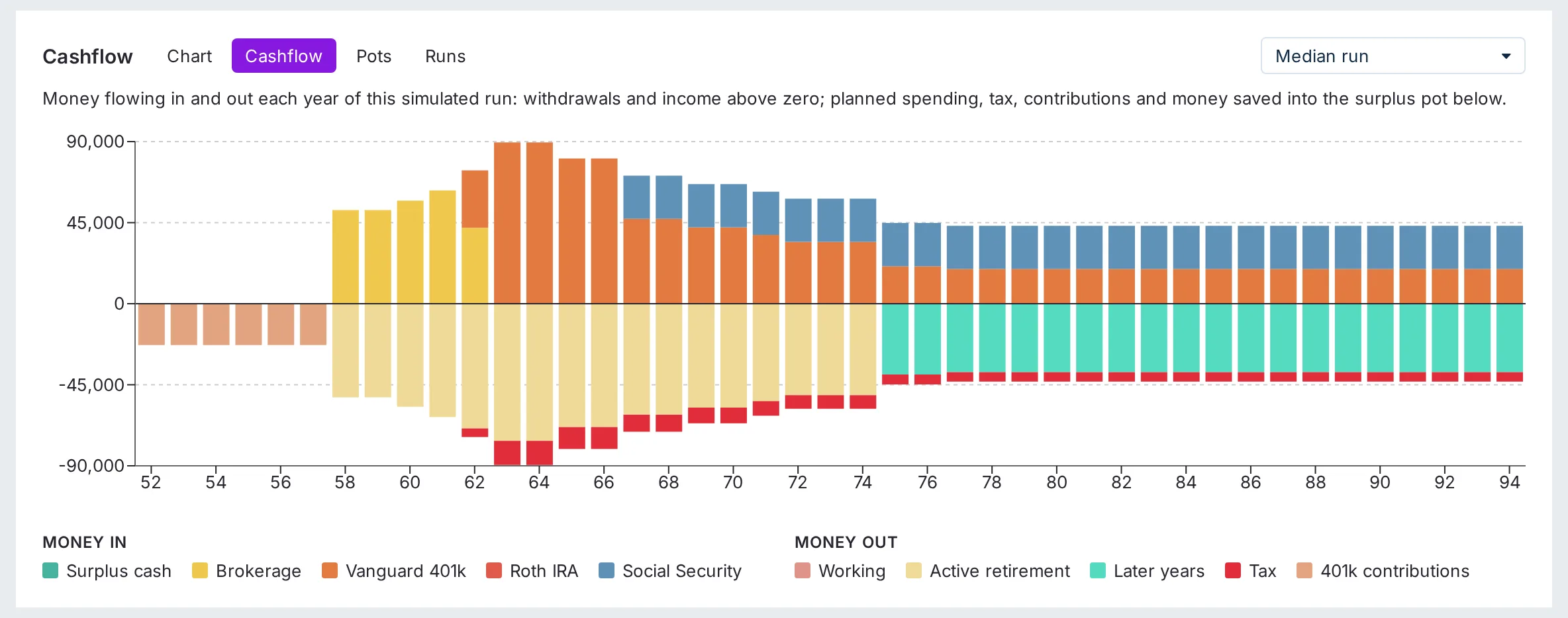
Switch the results view from Chart to Cashflow to see the money flowing through your hands each year, for one simulated run at a time:
- Above zero: money coming in - each pot's withdrawal for the year (one color per pot), plus each income stream (one color per stream).
- Below zero: money going out - the year's planned spending, colored by the spending phase it belongs to; the tax paid on withdrawals and income; each contribution being paid into a pot (one color per contribution); and money saved into your surplus pot, if you keep unspent money.
Management fees don't appear here - they are charged inside the pots and never pass through your hands, and the run detail table lists them. Income you didn't need shows up as inflows that outweigh the outflows, and the tooltip names the unspent amount.
On a run that fails, the chart doesn't stop at the failure year: the remaining years keep showing the spending the plan still called for, dimmed, with nothing coming in to fund it - so the size of the gap is visible at a glance. Those dimmed bars are held at the failure year's level - its price level, since a dead run no longer experiences inflation, and any cut or raise a withdrawal rule had in force at the time.
The spending bars show the plan - the phase amount, adjusted for inflation, any withdrawal rule and the minimum spending floor - rather than the money actually delivered. That's what makes trouble visible: in a shortfall year the withdrawal bars fall visibly short of the spending bar.
Use the dropdown above the chart to pick which run to look at: the worst run, a typically-bad or typically-good outcome (the 25th and 75th percentiles), the median, or the best run. These are the same runs the Jump to dropdown in the runs view lands on. The chart also appears above the year-by-year table when you click into any individual run, where Cashflow and Pots buttons switch between this chart and the pot balances chart.
The Pot Balances Chart
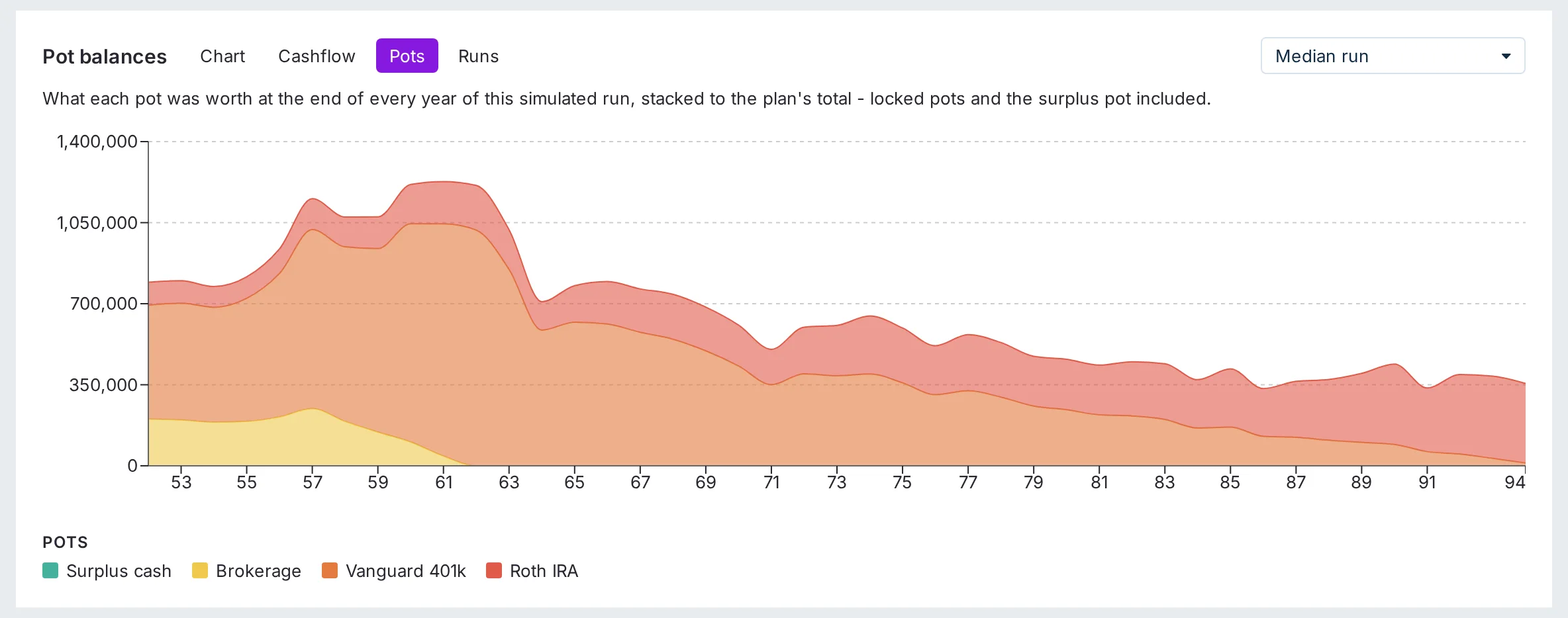
Switch the results view to Pots to see what each of your pots was worth at the end of every year, for one simulated run at a time. The pots are stacked on top of each other, one color per pot (the same colors as the cashflow chart), so the top of the stack is the plan's total balance and the bands inside it show how that total is split. Locked pots and the surplus pot are included, so you can watch a pension sit untouched until its access age, or the surplus pot fill up with income the plan didn't need.
Hover over a year to see every pot's balance and the total. On a run that fails, the accessible pots are emptied in the failure year - so the stack may not reach zero that year if money is still locked in a pot that hasn't reached its access age - and every year after it is drawn as zero.
The dropdown above the chart picks the run, exactly as it does for the cashflow chart, and the chart also appears above the year-by-year table when you click into a run from the Runs view, where Cashflow and Pots buttons switch between the two charts. Like every other figure in the results, the balances follow the Show values in today's money checkbox.
When Did the Pot Run Out?
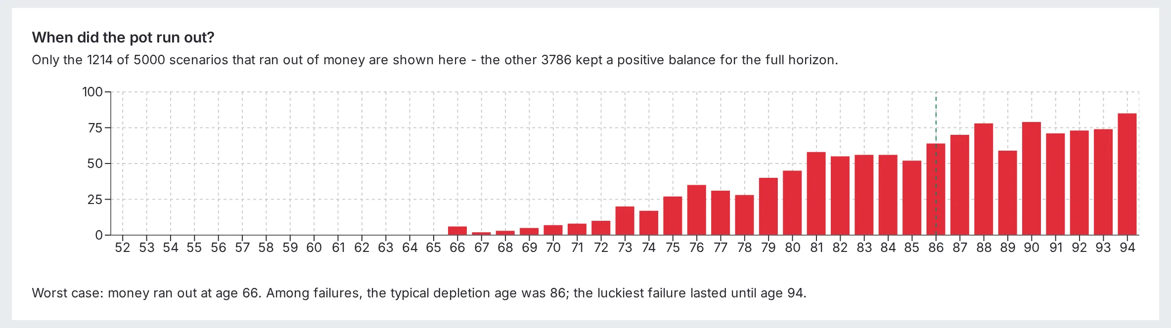
This bar chart only counts the replays that failed, showing at which age they ran out. If 900 of 5,000 replays failed, these bars add up to 900 - the other 4,100 kept a positive balance the whole way and don't appear here.
Exploring Individual Runs
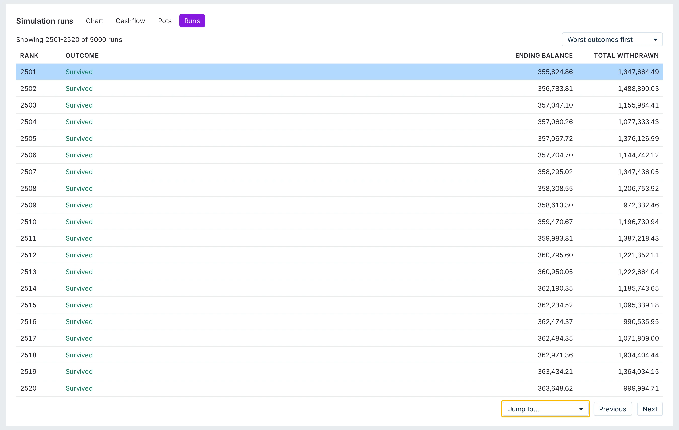
Switch the results view from Chart to Runs to see every replay listed from worst outcome to best. Rather than paging through thousands of runs, use the Jump to dropdown to go straight to the worst, median or best run - or the 25th/75th percentile for a typically-bad or typically-good outcome - with the run highlighted so you can click into it. Click any run to walk through it year by year: the balance at the start of each year, the contributions paid in (when your plan has any, including money saved into the Surplus cash pot), the net income received (when your plan has income streams), the withdrawal taken, what was actually spent (income and withdrawal together, net of tax - shown in red when it fell short of the plan), the investment growth in that year (as money and as a percentage), the year's inflation rate (when inflation is enabled), and the balance at the end. Expand a year with the arrow at the start of its row (or use Expand all years) and it opens with a short plain-English summary of what happened that year and why: any change the withdrawal rule made and what triggered it, whether the minimum spending floor stepped in, how the year's spending was funded (income, pots, or a shortfall), and where any money the plan didn't spend went. Below it sits the pot table described further down. Click Show the working for the fully labeled breakdown behind the summary: the income received, split into gross, tax and net (and per stream when you have several), with any unspent income called out; the withdrawal split into gross, tax and money to spend; how the year's spending compared with the plan (as planned, or short by an amount); when a withdrawal rule is active, a sentence showing how the rule arrived at that year's amount (and whether the minimum spending floor stepped in); the contributions added; the fees paid; and a small table showing each pot's balance at the start of the year, what it was invested in that year (when a pot has investment phases), what was contributed into it (for the Surplus cash pot, the money saved into it that year), what it contributed to the withdrawal, how much of that counted as taxable income, the tax paid on its share, the fee it was charged that year, its return that year, and its ending balance - so you can watch, for example, the cash pot covering spending after a crash while the stock pots are left alone. With the tax-bands model, the per-pot tax is the year's tax bill shared out in proportion to each pot's taxable income.
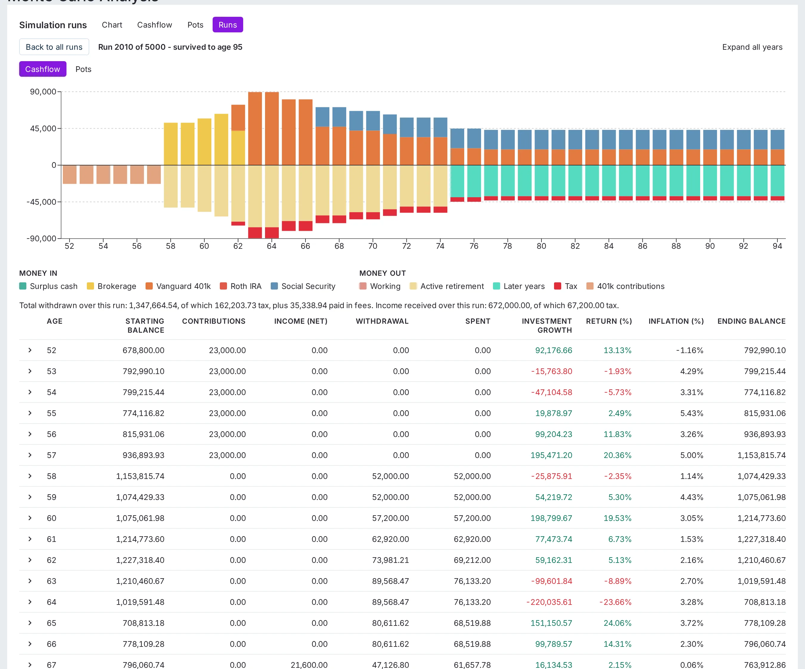
Above the year-by-year table, a summary line totals the run: how much was withdrawn over the whole replay, how much of that went to tax, how much was paid in fees on top, and - when the plan has income streams - how much income was received and the tax paid on it.
If a run failed while money was still locked in an inaccessible pot, the table says so explicitly, so you can tell the difference between "the market ate my savings" and "the money existed but I couldn't reach it yet."
Things to Keep in Mind
- This is a model, not a prophecy. A 90% success rate does not mean success is guaranteed - 1 in 10 of the simulated futures still failed.
- The random model is simplified. It draws each year independently, which ignores the way real crashes cluster together and the occasional extreme year. It also moves all pots in step - there's no independent luck per pot, so a bond-heavy pot dips a little in the same year a stock-heavy pot crashes. The historical models partly address the first point.
- The historical data is US market data (S&P 500 shares, US government bonds and bills, from 1928 onwards). US markets had an unusually good century, so results may be optimistic if your money is invested elsewhere.
- Investment phases switch for free. A pot that changes investments at an age, or glides between them, pays no dealing costs or tax on the switch. A gradual glide between hand-typed return and volatility figures moves both in a straight line, which slightly overstates the volatility of the in-between years.
- Fees and taxes are approximations you control. Each pot's fee settings model yearly costs explicitly - so enter expected returns gross of those fees to avoid double-counting - and the Tax settings are effective-rate estimates, not a tax calculator.
- Garbage in, garbage out. The results are only as good as your estimates for returns, volatility, spending and inflation. Try a few variations - small changes to the withdrawal often move the success rate a lot.