Excel Formula Mode (Formula cards & Rule formulas)
This is an experimental feature. That means we're still working on finishing it. There may be bugs, missing functionality or incomplete documentation, and we may decide to remove the feature in a future release. If you have any feedback, please comment on the dedicated feedback issue or post a message in the Discord.
All functionality described here may not be available in the latest stable release. See Experimental Features for instructions to enable experimental features. Use the nightly images for the latest implementation.
Excel formula mode adds two related features:
- Formula cards: a dashboard/report card that evaluates an Excel-style formula, including totals from custom queries.
- Rule formulas: in the Rules editor, some “set field” actions can be driven by a formula instead of a fixed value.
Under the hood, Actual evaluates formulas using HyperFormula. Formulas must start with =.
Enable the feature
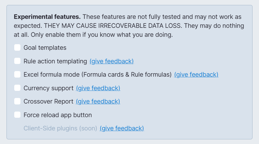
Go to Settings -> Show advanced settings -> Experimental features and enable:
- Excel formula mode (Formula cards & Rule formulas)
Formula cards
Add a Formula card
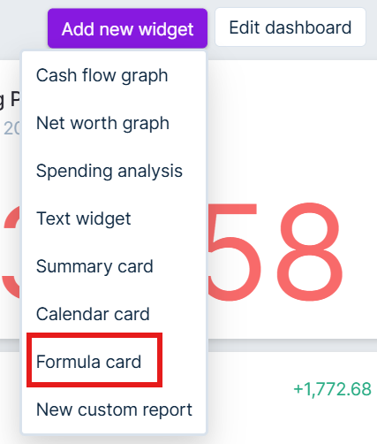
- Go to Reports
- Click Edit dashboard
- Click Add widget
- Choose Formula card
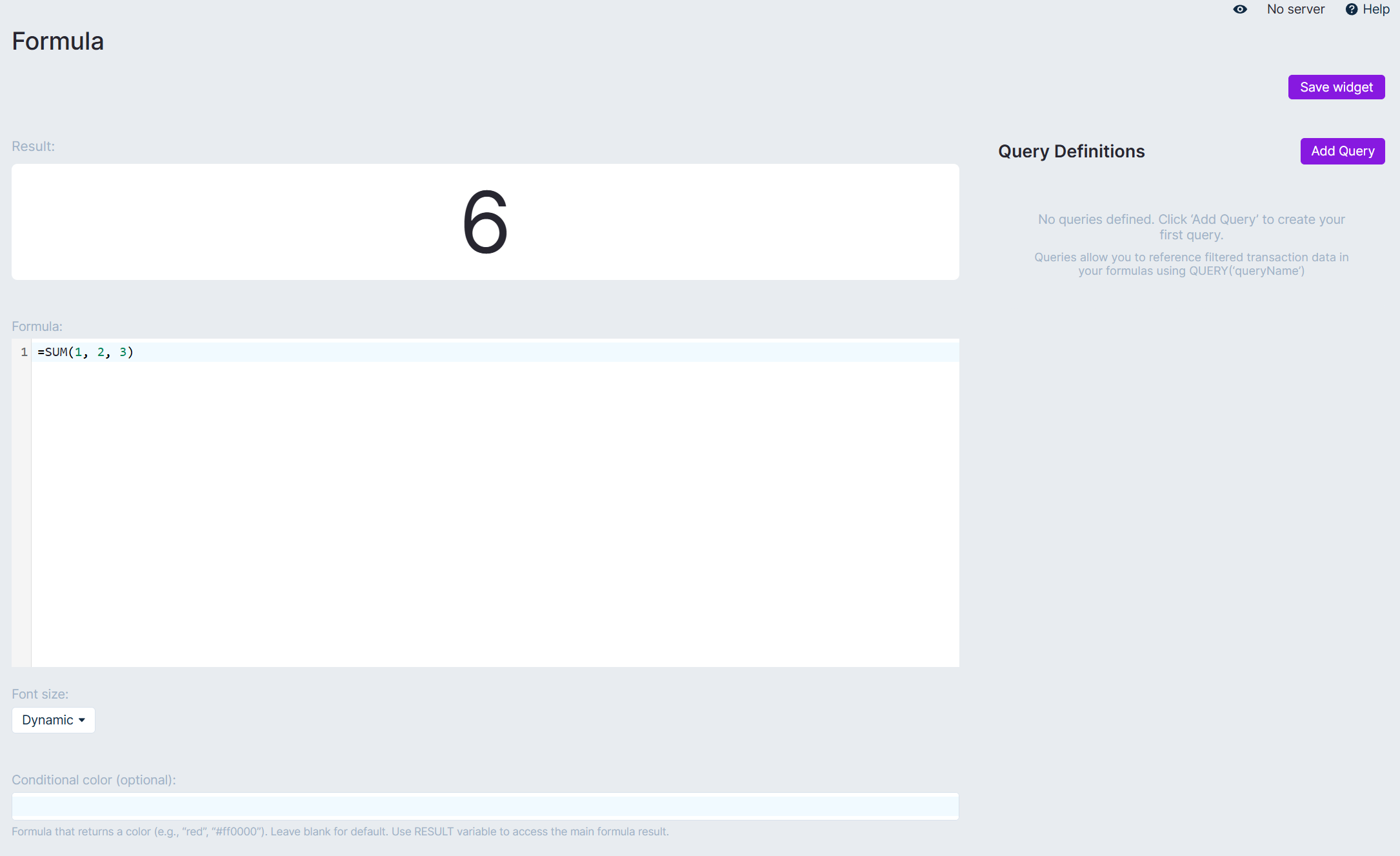
Click the card to open the editor (where you can save the widget).
Write a formula
- Start with
=(example:=SUM(1, 2, 3)) - You can use typical Excel-style functions (autocomplete and hover help are built into the editor).
Function reference
This list documents formula functions that are useful in Actual. The in-app autocomplete/hover popover provides a curated subset of these functions.
If a function isn’t listed here, it still might work. Actual uses HyperFormula under the hood, so you can also refer to HyperFormula’s built-in functions list.
| Function | Available in | Description | Syntax example | Optional params |
|---|---|---|---|---|
ABS | Query, Rules | Returns the absolute value of a number. | =ABS(-42) | — |
AND | Query, Rules | Returns TRUE if all arguments are TRUE. | =AND(1=1, 2=2) | Accepts more than 2 conditions |
AVERAGE | Query | Returns the average of all numbers in a range. | =AVERAGE(1, 2, 3) | Accepts more than 2 values |
AVERAGEA | Query | Returns the average, including text and logical values. | =AVERAGEA(1, TRUE, "2") | Accepts more than 2 values |
BALANCE_OF | Rules | Returns running balance for another account in cents; pass a quoted account id or exact account name. | =BALANCE_OF("550e8400-e29b-41d4-a716-446655440000"); =BALANCE_OF("Checking") | — |
BUDGET_QUERY | Query | Returns a budget dimension total for a set of categories over a month range. Dimension is one of: budgeted, spent, balance_start, balance_end, goal. | =BUDGET_QUERY("spent", QUERY_EXTRACT_CATEGORIES("q"), QUERY_EXTRACT_TIMEFRAME_START("q"), QUERY_EXTRACT_TIMEFRAME_END("q")) | — |
CEILING | Query, Rules | Rounds up to nearest multiple of significance. | =CEILING(10.2, 1) | — |
CHAR | Query, Rules | Converts number to character. | =CHAR(65) | — |
CHOOSE | Query | Returns value from list based on index. | =CHOOSE(2, "A", "B", "C") | Accepts more than 2 values |
CLEAN | Rules | Removes non-printable characters from text. | =CLEAN(notes) | — |
CODE | Query, Rules | Returns numeric code for first character. | =CODE("A") | — |
CONCATENATE | Query, Rules | Combines several text strings into one. | =CONCATENATE("Paid ", payee_name) | Accepts more than 2 texts |
COS | Query | Returns the cosine of an angle. | =COS(1) | — |
COUNT | Query | Counts the number of numeric values. | =COUNT(1, 2, "x") | Accepts more than 2 values |
COUNTA | Query | Counts non-empty values. | =COUNTA(1, "", "x") | Accepts more than 2 values |
COUNTBLANK | Query | Counts empty cells. | =COUNTBLANK(A1:A10) | — |
COUNTIF | Query | Counts cells that meet a criteria. | =COUNTIF(A1:A10, ">0") | — |
COUNTIFS | Query | Counts cells that meet multiple criteria. | =COUNTIFS(A1:A10, ">0", B1:B10, "<=5") | Repeat (range, criteria) pairs |
DATE | Query, Rules | Returns date as number of days since null date. | =DATE(2025, 12, 16) | — |
DATEDIF | Query, Rules | Calculates distance between dates. | =DATEDIF("2025-01-01", "2025-12-31", "D") | — |
DATEVALUE | Rules | Parses a date string and returns it as a number. | =DATEVALUE("2025-12-16") | — |
DAY | Query, Rules | Returns the day from a date. | =DAY(date) | — |
DAYS | Query, Rules | Calculates difference between dates in days. | =DAYS("2025-12-31", "2025-12-01") | — |
EDATE | Query, Rules | Returns date shifted by specified months. | =EDATE(date, 1) | — |
EOMONTH | Query, Rules | Returns last day of month after specified months. | =EOMONTH(date, 0) | — |
EXACT | Query, Rules | Returns TRUE if texts are exactly the same. | =EXACT("A", "a") | — |
EXP | Query | Returns e raised to the power of number. | =EXP(1) | — |
FALSE | Query, Rules | Returns the logical value FALSE. | =FALSE() | — |
FIND | Query, Rules | Finds text within text (case-sensitive). | =FIND("foo", notes) | — |
FLOOR | Query, Rules | Rounds down to nearest multiple of significance. | =FLOOR(10.8, 1) | — |
FORMATCURRENCY | Query, Rules | Formats a number as currency using your app currency, number format, symbol position, and spacing settings by default. | =FORMATCURRENCY(1234.5) | symbol, decimals, thousandsSeparator, decimalSeparator, symbolPosition, spaceBetweenAmountAndSymbol |
FORMATNUMBER | Query, Rules | Formats a number using your app number format settings by default. | =FORMATNUMBER(1234.5, 2) | decimals, thousandsSeparator, decimalSeparator |
FV | Query | Calculates future value of investment. | =FV(0.05/12, 12, -100) | — |
HLOOKUP | Query | Searches horizontally in first row and returns value. | =HLOOKUP("key", A1:D10, 2, TRUE) | — |
IF | Query, Rules | Returns one value if condition is TRUE, another if FALSE. | =IF(amount<0, "Expense", "Income") | — |
IFERROR | Query, Rules | Returns value if no error, otherwise returns alternative. | =IFERROR(1/0, 0) | — |
IFNA | Query, Rules | Returns value if not #N/A error, otherwise returns alternative. | =IFNA(VLOOKUP("x", A1:B10, 2, FALSE), 0) | — |
IFS | Query, Rules | Checks multiple conditions and returns corresponding values. | =IFS(amount<0, "Expense", amount>0, "Income") | Repeat (condition, value) pairs |
INDEX | Query | Returns value at specified row and column. | =INDEX(A1:C10, 2, 3) | — |
INTEGER_TO_AMOUNT | Query, Rules | Converts integer amount to decimal amount (e.g., 1234 -> 12.34). | =INTEGER_TO_AMOUNT(amount, 2) | decimal_places (default: 2) |
INT | Rules | Rounds down to nearest integer. | =INT(10.9) | — |
IRR | Query | Calculates internal rate of return. | =IRR(A1:A12) | — |
ISEVEN | Rules | Returns TRUE if number is even. | =ISEVEN(10) | — |
ISODD | Rules | Returns TRUE if number is odd. | =ISODD(11) | — |
ISBLANK | Query, Rules | Returns TRUE if value is blank. | =ISBLANK(notes) | — |
ISERROR | Query, Rules | Returns TRUE if value is any error. | =ISERROR(1/0) | — |
ISLOGICAL | Query, Rules | Returns TRUE if value is logical (TRUE/FALSE). | =ISLOGICAL(TRUE()) | — |
ISNA | Query, Rules | Returns TRUE if value is #N/A error. | =ISNA(NA()) | — |
ISNUMBER | Query, Rules | Returns TRUE if value is a number. | =ISNUMBER(amount) | — |
ISOWEEKNUM | Rules | Returns ISO week number. | =ISOWEEKNUM(date) | — |
ISREF | Query, Rules | Returns TRUE if value is a reference. | =ISREF(A1) | — |
ISTEXT | Query, Rules | Returns TRUE if value is text. | =ISTEXT(notes) | — |
LEFT | Query, Rules | Returns leftmost characters from text. | =LEFT(imported_payee, 10) | — |
LEN | Query, Rules | Returns length of text. | =LEN(notes) | — |
LN | Query | Returns the natural logarithm. | =LN(10) | — |
LOG | Query | Returns the logarithm to specified base. | =LOG(100, 10) | — |
LOG10 | Query | Returns the base-10 logarithm. | =LOG10(1000) | — |
LOOKUP | Query | Looks up values in a vector or array. | =LOOKUP("x", A1:A10) | — |
LOWER | Query, Rules | Converts text to lowercase. | =LOWER(notes) | — |
MATCH | Query | Returns position of value in array. | =MATCH("x", A1:A10, 0) | — |
MAX | Query | Returns the maximum value. | =MAX(1, 2, 3) | Accepts more than 2 values |
MAXA | Query | Returns the maximum value, including text and logical values. | =MAXA(1, TRUE, "2") | Accepts more than 2 values |
MEDIAN | Query | Returns the median value. | =MEDIAN(1, 2, 100) | Accepts more than 2 values |
MID | Query, Rules | Returns substring from specified position. | =MID(notes, 1, 10) | — |
MIN | Query | Returns the minimum value. | =MIN(1, 2, 3) | Accepts more than 2 values |
MINA | Query | Returns the minimum value, including text and logical values. | =MINA(1, TRUE, "2") | Accepts more than 2 values |
MOD | Query, Rules | Returns the remainder of division. | =MOD(10, 3) | — |
MODE | Query | Returns the most frequently occurring value. | =MODE(1, 1, 2) | Accepts more than 2 values |
MONTH | Query, Rules | Returns the month from a date. | =MONTH(date) | — |
N | Rules | Converts value to a number. | =N(TRUE()) | — |
NETWORKDAYS | Query | Returns number of working days between dates. | =NETWORKDAYS("2025-12-01", "2025-12-31") | — |
NOT | Query, Rules | Reverses the logical value. | =NOT(amount<0) | — |
NOW | Query, Rules | Returns current date and time. | =NOW() | — |
NPV | Query | Calculates net present value. | =NPV(0.1, -1000, 200, 300) | Accepts more than 2 values |
OR | Query, Rules | Returns TRUE if any argument is TRUE. | =OR(amount<0, amount>0) | Accepts more than 2 conditions |
PERCENTILE | Query | Returns the k-th percentile. | =PERCENTILE(A1:A100, 0.9) | — |
PI | Query | Returns the value of PI. | =PI() | — |
PMT | Query | Calculates payment for a loan. | =PMT(0.05/12, 60, 10000) | — |
POWER | Query, Rules | Returns base raised to the power of exponent. | =POWER(2, 8) | — |
PROPER | Query, Rules | Capitalizes first letter of each word. | =PROPER(notes) | — |
PRODUCT | Query | Returns the product of all numbers. | =PRODUCT(2, 3, 4) | Accepts more than 2 values |
PV | Query | Calculates present value of investment. | =PV(0.05/12, 12, -100) | — |
QUARTILE | Query | Returns the quartile of a dataset. | =QUARTILE(A1:A100, 1) | — |
QUERY | Query | Execute a query and return the result. | =QUERY("expenses") | — |
QUERY_COUNT | Query | Execute a query and return the number of matching rows. | =QUERY_COUNT("expenses") | — |
QUERY_EXTRACT_CATEGORIES | Query | Determines which categories to include based on a named query's category filters; used as the categories argument in BUDGET_QUERY. | =QUERY_EXTRACT_CATEGORIES("expenses") | — |
QUERY_EXTRACT_TIMEFRAME_END | Query | Extracts the end month from a named query's date range; used as the endMonth argument in BUDGET_QUERY. | =QUERY_EXTRACT_TIMEFRAME_END("expenses") | — |
QUERY_EXTRACT_TIMEFRAME_START | Query | Extracts the start month from a named query's date range; used as the startMonth argument in BUDGET_QUERY. | =QUERY_EXTRACT_TIMEFRAME_START("expenses") | — |
RANK | Query | Returns the rank of a number in a list. | =RANK(10, A1:A10, 0) | — |
RATE | Query | Calculates interest rate per period. | =RATE(60, -200, 10000) | — |
REPLACE | Query, Rules | Replaces substring at specified position. | =REPLACE(notes, 1, 5, "") | — |
REPT | Query, Rules | Repeats text specified number of times. | =REPT("*", 10) | — |
RIGHT | Query, Rules | Returns rightmost characters from text. | =RIGHT(imported_payee, 4) | — |
ROUND | Query, Rules | Rounds a number to specified decimals. | =ROUND(amount/100, 2) | — |
ROUNDDOWN | Query, Rules | Rounds down to specified decimals. | =ROUNDDOWN(amount/100, 0) | — |
ROUNDUP | Query, Rules | Rounds up to specified decimals. | =ROUNDUP(amount/100, 0) | — |
SEARCH | Query, Rules | Finds text within text (case-insensitive, supports wildcards). | =SEARCH("foo", notes) | — |
SIGN | Rules | Returns -1 for negative, 0 for zero, 1 for positive. | =SIGN(amount) | — |
SIN | Query | Returns the sine of an angle. | =SIN(1) | — |
SPLIT | Rules | Splits text by space and returns part at index. | =SPLIT(imported_payee, 0) | — |
SQRT | Query, Rules | Returns the square root. | =SQRT(9) | — |
STDEV | Query | Returns the standard deviation of a sample. | =STDEV(A1:A10) | — |
STDEVP | Query | Returns the standard deviation of a population. | =STDEVP(A1:A10) | — |
SUBSTITUTE | Query, Rules | Replaces occurrences of text. | =SUBSTITUTE(imported_payee, " 12345", "") | — |
SUM | Query, Rules | Returns the sum of all numbers in a range. | =SUM(1, 2, 3) | Accepts more than 2 values |
SUMIF | Query | Sums cells that meet a criteria. | =SUMIF(A1:A10, ">0", B1:B10) | — |
SUMIFS | Query | Sums cells that meet multiple criteria. | =SUMIFS(B1:B10, A1:A10, ">0", C1:C10, "X") | Repeat (range, criteria) pairs |
SUMPRODUCT | Query | Multiplies corresponding elements and returns the sum. | =SUMPRODUCT(A1:A10, B1:B10) | Accepts more arrays |
SUMSQ | Query | Returns the sum of the squares. | =SUMSQ(1, 2, 3) | Accepts more than 2 values |
SWITCH | Query, Rules | Matches expression against values and returns corresponding result. | =SWITCH(category_name, "Groceries", "Food", "Fuel", "Transport") | Repeat (value, result) pairs; default supported |
T | Rules | Returns text if value is text, empty string otherwise. | =T(notes) | — |
TAN | Query | Returns the tangent of an angle. | =TAN(1) | — |
TEXT | Query, Rules | Converts number to text with format. | =TEXT(date, "MMMM yyyy") | — |
TODAY | Query, Rules | Returns current date. | =TODAY() | — |
TRIM | Query, Rules | Removes extra spaces from text. | =TRIM(notes) | — |
TRUNC | Rules | Truncates number to specified decimals. | =TRUNC(amount/100, 0) | — |
TRUE | Query, Rules | Returns the logical value TRUE. | =TRUE() | — |
UPPER | Query, Rules | Converts text to uppercase. | =UPPER(notes) | — |
VALUE | Rules | Converts text to a number. | =VALUE("123.45") | — |
VAR | Query | Returns the variance of a sample. | =VAR(A1:A10) | — |
VARP | Query | Returns the variance of a population. | =VARP(A1:A10) | — |
VLOOKUP | Query | Searches vertically in first column and returns value. | =VLOOKUP("key", A1:D10, 2, TRUE) | — |
WEEKDAY | Query, Rules | Returns day of week (1-7). | =WEEKDAY(date, 1) | — |
WEEKNUM | Query, Rules | Returns week number of year. | =WEEKNUM(date, 1) | — |
XOR | Query, Rules | Returns TRUE if odd number of arguments are TRUE. | =XOR(TRUE(), FALSE()) | Accepts more than 2 conditions |
YEAR | Query, Rules | Returns the year from a date. | =YEAR(date) | — |
Formatting numbers and currency
FORMATNUMBER and FORMATCURRENCY use your app formatting preferences when optional arguments are omitted.
=FORMATNUMBER(1234.5, 2)
=FORMATCURRENCY(1234.5)
You can override separators and currency display for a single formula:
=FORMATCURRENCY(1234.5, "€", 2, ".", ",", "after", TRUE())
The symbolPosition argument accepts "before" or "after". The spaceBetweenAmountAndSymbol argument accepts TRUE() or FALSE().
Use queries with QUERY("name") and QUERY_COUNT("name")
Formula cards can reference named queries that you define in the right-side panel (Query Definitions).
QUERY("myQuery")returns the sum of transaction amounts for that query’s filters and date range (returned in normal “money” units, e.g.-123.45).- If a query name doesn’t exist, it evaluates as 0.
Example:
=QUERY("income") - QUERY("expenses")
Define a query
In the Formula editor page, use Query Definitions:
- Add Query and give it a name (the name is what you reference in
QUERY("...")) - Set the date range:
- Live: keeps the range moving (e.g. “last 3 months”)
- Static: fixed start/end dates
- Add Filters (same style as report filters)
Budget queries with BUDGET_QUERY
BUDGET_QUERY reads directly from your envelope budget (budgeted amounts, spending, balances, and goals) for a fixed set of categories over a month range.
Syntax:
=BUDGET_QUERY("dimension", categories, startMonth, endMonth)
| Parameter | Description |
|---|---|
dimension | What to return. One of: budgeted, spent, balance_start, balance_end, goal |
categories | Which categories to include — use QUERY_EXTRACT_CATEGORIES("queryName") to pull from a named query's filters. Advanced: a literal array of category IDs ({"id1";"id2"}) is also accepted, but using the extract function is recommended. |
startMonth | Start month in YYYY-MM format, or QUERY_EXTRACT_TIMEFRAME_START("queryName") |
endMonth | End month in YYYY-MM format, or QUERY_EXTRACT_TIMEFRAME_END("queryName") |
The result is in normal "money" units (e.g. -123.45), the same as QUERY().
Dimension reference:
| Dimension | Description |
|---|---|
budgeted | Total amount budgeted across the month range |
spent | Total amount spent (sum of transactions) across the month range |
balance_start | Carryover balance at the start of the first month (leftover from the prior month) |
balance_end | Running balance at the end of the last month (budgeted + spent + carryover) |
goal | Total goal amount across the month range |
Using QUERY_EXTRACT_* helpers
These three helpers pull values out of a named query definition so you can reuse a query's filters and date range as inputs to BUDGET_QUERY:
QUERY_EXTRACT_CATEGORIES("queryName")— uses the query's category filters to determine which categories to include. If the query has no category filter, all non-income, non-hidden categories are included.QUERY_EXTRACT_TIMEFRAME_START("queryName")— returns the query's start month as aYYYY-MMstring.QUERY_EXTRACT_TIMEFRAME_END("queryName")— returns the query's end month as aYYYY-MMstring.
Example — total spent for the same categories and date range as a named query called expenses:
=BUDGET_QUERY("spent", QUERY_EXTRACT_CATEGORIES("expenses"), QUERY_EXTRACT_TIMEFRAME_START("expenses"), QUERY_EXTRACT_TIMEFRAME_END("expenses"))
Example — compare budgeted vs actual spent for a hard-coded month range:
=BUDGET_QUERY("budgeted", QUERY_EXTRACT_CATEGORIES("expenses"), "2025-01", "2025-03")
  - BUDGET_QUERY("spent", QUERY_EXTRACT_CATEGORIES("expenses"), "2025-01", "2025-03")
Optional: conditional color
Formula cards support an optional Conditional color formula (single line) that returns a color string like red or #ff0000.
- Use the
RESULTvariable to reference the main formula result.
Rule formulas
Rule formulas let you compute a value from the current transaction and set a field to that computed result.
Note: rule formula inputs are single-line (line breaks are automatically replaced with spaces).
Where to find the formula toggle
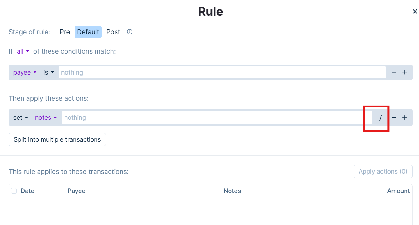
In More -> Rules -> edit a rule, on a Set action:
- Click the ƒ button to the right of the action input to enable/disable formula mode for that action.
- Formula mode is not available for actions that set payee, category, or account (those values are IDs).
- Rule action templating (the
</>icon) and formulas are mutually exclusive: enabling one disables the other.
Available variables
Rule formulas evaluate with named variables from the transaction context, including:
Date variables:
today— Current date in YYYY-MM-DD format (e.g.,"2025-12-19")date— Transaction date in YYYY-MM-DD format (e.g.,"2025-01-15")
Numeric variables (stored in cents):
amount— Transaction amount as an integer in cents (e.g.,12345represents $123.45)- Positive for income, negative for expenses
- To convert to dollars:
=amount / 100
balance— Account balance after this transaction, as an integer in cents- Represents the running balance at this transaction
- To convert to dollars:
=balance / 100
Text variables:
notes— Transaction notes/memo field (string, may be empty)imported_payee— Original payee name from import before any rules applied (string)payee_name— Resolved payee name (string)account_name— Account name where transaction exists (string)category_name— Category name assigned to transaction (string)
Boolean variables:
cleared— Whether transaction is cleared (TRUEorFALSE)reconciled— Whether transaction is reconciled (TRUEorFALSE)
Tip: if you want “dollars” from amount, use =amount / 100.
Available functions
BALANCE_OF (other accounts):
=BALANCE_OF("550e8400-e29b-41d4-a716-446655440000")
=BALANCE_OF("Checking")
BALANCE_OF("…")— Running balance for another account, in cents, using the same cutoff asbalance(samedate,sort_order, andidordering as the current transaction).- Pass a quoted account id (matches an account id in your budget) for a deterministic result, or a quoted account name for an exact name match. If the account name is ambiguous (duplicates), the first match is used.
- If the account is not found, the value is 0.
- For the current transaction’s account, use the
balancevariable instead ofBALANCE_OF. - Returns an integer in cents. For the amount in dollars, divide by 100 or
=INTEGER_TO_AMOUNT(BALANCE_OF("Checking")).
Result types
When a rule runs, Actual converts the formula result to the field type:
- number fields: must produce a number (or a string that parses as a number)
- date fields: must produce a valid date
- boolean fields:
TRUE/FALSE(or a string that equals"true"/"false") - string fields: converted with
String(...)